
Table of Contents
Introduction
Regression analysis is a powerful statistical tool used to model and analyze relationships between variables. It involves fitting a mathematical model to observed data to understand and predict the behaviour of one variable based on the values of another or multiple variables. In this paper, we delve into the concepts of simple linear regression, the principle of least squares, and the fitting of polynomials and exponential curves, along with real-life examples to illustrate their applications.
Simple Linear Regression
Simple linear regression aims to find a linear relationship between two variables, typically denoted as the dependent variable ( ) and the independent variable (
 ). The equation for simple linear regression is given by:
![\[ y = \beta_0 + \beta_1 x + \varepsilon \]](https://360studies.com/wp-content/ql-cache/quicklatex.com-24b9be760189aa8ba22294b2f9529a4b_l3.png "Rendered by QuickLaTeX.com")
where  is the y-intercept,
  is the slope of the line, and
  represents the error term.
Principle of least squares method
The principle of least squares is a mathematical method used in regression analysis to find the best-fitting line or curve that explains the relationship between the variables in a dataset. It minimizes the sum of the squared differences between the observed data points and the values predicted by the regression model.
Let’s consider a simple linear regression model, where we have a set of  data points
  , and we want to find the best-fitting line
  that predicts based on .
The difference between the observed  and the predicted
  values for each data point is given by the residual
  :
:
![\[ \varepsilon_i = y_i - y_{\text{pred},i} \]](https://360studies.com/wp-content/ql-cache/quicklatex.com-2706004dcc4b106e5756a4b5de1f0008_l3.png "Rendered by QuickLaTeX.com")
The goal is to minimize the sum of the squared residuals for all data points:
![\[ S = \sum_{i=1}^{n} \varepsilon_i^2 = \sum_{i=1}^{n} (y_i - y_{\text{pred},i})^2 \]](https://360studies.com/wp-content/ql-cache/quicklatex.com-752d570f32fa82f85d5d75dc2fcc870f_l3.png "Rendered by QuickLaTeX.com")
This is the sum of squared differences between the observed and the predicted values. The principle of least squares seeks to find the values of and that minimize this sum  .
.
Mathematically, we want to find and that satisfy:
![\[ \min_{\beta_0, \beta_1} \sum_{i=1}^{n} (y_i - (\beta_0 + \beta_1 x_i))^2 \]](https://360studies.com/wp-content/ql-cache/quicklatex.com-22d61a9e5eb56ddf0898535d60b4d818_l3.png "Rendered by QuickLaTeX.com")
To find the minimum, we take the partial derivatives of the sum with respect to and , set them to zero, and solve for and .
Taking the partial derivative with respect to :
![\[ \frac{\partial S}{\partial \beta_0} = -2 \sum_{i=1}^{n} (y_i - (\beta_0 + \beta_1 x_i)) = 0 \]](https://360studies.com/wp-content/ql-cache/quicklatex.com-9048129354ec76ddbe738f7fd8ec6795_l3.png "Rendered by QuickLaTeX.com")
Taking the partial derivative with respect to :
![\[ \frac{\partial S}{\partial \beta_1} = -2 \sum_{i=1}^{n} x_i (y_i - (\beta_0 + \beta_1 x_i)) = 0 \]](https://360studies.com/wp-content/ql-cache/quicklatex.com-27a29954c459ecffc78bdf3f73b79fda_l3.png "Rendered by QuickLaTeX.com")
Solving these equations simultaneously gives the optimal values for and that minimize the sum of squared residuals.
The final equations for and are:
![\[ \beta_1 = \frac{n \sum x_i y_i - \sum x_i \sum y_i}{n \sum x_i^2 - (\sum x_i)^2} \]](https://360studies.com/wp-content/ql-cache/quicklatex.com-ead6bc6372032238ebde7ab0eb2cf67f_l3.png "Rendered by QuickLaTeX.com")
![\[ \beta_0 = \frac{\sum y_i - \beta_1 \sum x_i}{n} \]](https://360studies.com/wp-content/ql-cache/quicklatex.com-0ece597f56b41ba23506284cceecc48d_l3.png "Rendered by QuickLaTeX.com")
These equations ensure that the best-fitting line minimizes the sum of squared residuals and captures the linear relationship between the variables and .
In summary, the principle of least squares is a fundamental concept in regression analysis that aims to find the optimal parameters of a regression model by minimizing the sum of squared differences between observed and predicted values. This method results in the best-fitting line that represents the relationship between variables in the dataset.
Real-life Example: House Prices
Consider a real estate scenario where you want to predict house prices () based on their size (). By collecting data on house sizes and corresponding prices, you can perform simple linear regression to find the best-fitting line that predicts prices based on house sizes.
Python Code :
import numpy as np
import matplotlib.pyplot as plt
from sklearn.linear_model import LinearRegression

# Generating example data
np.random.seed(0)
hours_studied = np.random.randint(1, 10, 20)
final_scores = 50 + 5 * hours_studied + np.random.normal(0, 5, 20)

# Reshaping data
hours_studied = hours_studied.reshape(-1, 1)
final_scores = final_scores.reshape(-1, 1)

# Creating a linear regression model
model = LinearRegression()

# Fitting the model
model.fit(hours_studied, final_scores)

# Predicting scores for new data
new_hours = np.array([[8]])
predicted_scores = model.predict(new_hours)

# Plotting the data and regression line
plt.scatter(hours_studied, final_scores, color='blue', label='Data')
plt.plot(hours_studied, model.predict(hours_studied), color='red', label='Regression Line')
plt.scatter(new_hours, predicted_scores, color='green', label='Predicted')
plt.xlabel('Hours Studied')
plt.ylabel('Final Exam Score')
plt.title('Linear Regression Example')
plt.legend()
plt.show()

print(f"Predicted score for {new_hours[0][0]} hours of studying: {predicted_scores[0][0]}")
Certainly! Let’s go through the provided Python code step by step and explain what each part does:
import numpy as np
import matplotlib.pyplot as plt
from sklearn.linear_model import LinearRegression
Here, we’re importing the necessary libraries: `numpy` for numerical operations, `matplotlib.pyplot` for data visualization, and `LinearRegression` from the `sklearn.linear_model` module for performing linear regression.
np.random.seed(0)
hours_studied = np.random.randint(1, 10, 20)
final_scores = 50 + 5 * hours_studied + np.random.normal(0, 5, 20)
Setting the random seed ensures that the random numbers generated are the same every time the code is run. This helps in reproducibility. We’re generating random data for the number of hours studied and simulating final exam scores. The final scores are generated using a linear equation ( ) with added noise using `np.random.normal()`.
hours_studied = hours_studied.reshape(-1, 1)
final_scores = final_scores.reshape(-1, 1)
Reshaping the data is necessary to match the expected format by the `LinearRegression` model. The data should be in a 2D array where each row corresponds to a sample, and each column corresponds to a feature.
model = LinearRegression()Creating an instance of the `LinearRegression` model.
model.fit(hours_studied, final_scores)Fitting the linear regression model to the data. This step calculates the optimal parameters (slope and intercept) for the linear relationship between hours studied and final scores.
new_hours = np.array([[8]])
predicted_scores = model.predict(new_hours)
Predicting the final exam score for a new value of hours studied (8 in this case) using the trained model.
plt.scatter(hours_studied, final_scores, color='blue', label='Data')
plt.plot(hours_studied, model.predict(hours_studied), color='red', label='Regression Line')
plt.scatter(new_hours, predicted_scores, color='green', label='Predicted')
plt.xlabel('Hours Studied')
plt.ylabel('Final Exam Score')
plt.title('Linear Regression Example')
plt.legend()
plt.show()
Plotting the data points as blue dots, the calculated regression line as a red line, and the predicted score for the new hours studied as a green dot. This visualizes how well the regression line fits the data and the predicted score for the new input.
print(f"Predicted score for {new_hours[0][0]} hours of studying: {predicted_scores[0][0]}")Printing out the predicted final exam score for the specified number of hours studied.
In summary, this code generates example data, performs linear regression using the `LinearRegression` model from `scikit-learn`, plots the data points, regression line, and predicted point, and displays the predicted score. This is a simple example to demonstrate how linear regression can be applied to real-world data using Python.
Output :
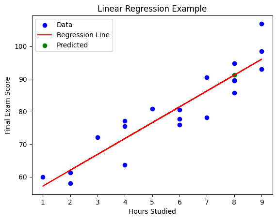
Predicted score for 8 hours of studying: 91.1369030821732Fitting Polynomials and Exponential Curves
While linear regression is suitable for linear relationships, many real-world scenarios involve more complex relationships that can be better modeled using polynomial or exponential curves.
Fitting Polynomials
Polynomial regression involves fitting a polynomial equation to the data. The general equation for polynomial regression of degree  is:
is:
![\[ y = \beta_0 + \beta_1 x + \beta_2 x^2 + \ldots + \beta_k x^k + \varepsilon \]](https://360studies.com/wp-content/ql-cache/quicklatex.com-142e1249c005c98178439d4180b28b79_l3.png "Rendered by QuickLaTeX.com")
Fitting Exponential Curves
Exponential regression is used when the relationship between variables can be better represented by an exponential equation. The general equation for exponential regression is:
![\[ y = \beta_0 e^{\beta_1 x} + \varepsilon \]](https://360studies.com/wp-content/ql-cache/quicklatex.com-137cf0c669eb0ac612171691a1883de5_l3.png "Rendered by QuickLaTeX.com")
Real-life Example: Population Growth
Consider a population growth scenario where you want to model the growth of a bacterial population () over time (). Exponential regression can be used to find the best-fitting exponential curve that describes the growth pattern.
Python Code:
import numpy as np
years = np.array([0, 1, 2, 3, 4, 5])
population = np.array([100, 150, 225, 338, 507, 761])
import matplotlib.pyplot as plt
from scipy.optimize import curve_fit

def exponential_curve(x, a, b):
return a * np.exp(b * x)

params, covariance = curve_fit(exponential_curve, years, population)

a_fit, b_fit = params

print("Fitted Parameters:")
print("a:", a_fit)
print("b:", b_fit)

# Plot the original data and the fitted exponential curve
plt.scatter(years, population, label='Original Data')
plt.plot(years, exponential_curve(years, a_fit, b_fit), color='red', label='Fitted Exponential Curve')
plt.xlabel('Years')
plt.ylabel('Population')
plt.legend()
plt.title('Exponential Curve Fitting')
plt.show()
Output :
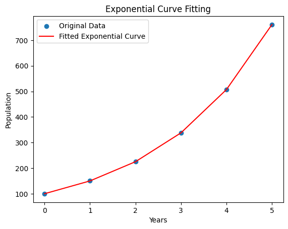
Fitted Parameters: a: 99.95044925069982 b: 0.4059889459865304